Blogs
Anja Raznjevic – Modeling dispersion of methane
Blog written by Anja Raznjevic
Modeling dispersion of methane (CH4) on the small scale is my main research topic and I work at Wageningen University (WUR), the Netherlands. For simulations I use Computational Fluid Dynamics (CFD) model called MicroHH, developed by Chiel van Heerwaarden et al. (for more information see http://microhh.org/), which simulates turbulent flows. MicroHH is designed for Direct Numerical Simulations (DNS) but can also support Large Eddy Simulations (LES), which means that, in the case of DNS, the turbulence is fully resolved and even the smallest eddies are captured, or in the case of LES, as its name says, the code simulates large turbulent eddies while the smallest eddies are parametrized. When it comes to measuring CH4close to the source, which many of the other PhD students are doing, the plume is transported by the turbulent flow and behaves in the same way as the flow does so these simulations can help with interpreting the measurement results and planning future measuring campaigns.
During my PhD I am supposed to have only one longer secondment, and that was to Empa, Switzerland. In my opinion, the secondments are a nice way to get to know other research groups, see how other scientific groups are functioning, meet new people, but still be with friends from the project that you got to know during schools and workshops. And I looked forward to seeing the Switzerland, which I never visited before.
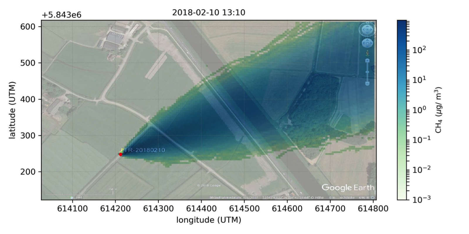
From the research perspective, I was really exited to get to see how a different kind of dispersion model works. At Empa they use the GRAL model, which is a Lagrangian particle dispersion model that simulates dispersion of non-reactive pollutants. In this model the flow and turbulence fields are obtained by solving Reynolds-averaged Navier Stokes (RANS) equations using k-ε turbulence closure. This means that while solving the same set of equations that MicroHH does, GRAL parametrizes the whole turbulent behavior and the transport of particles happens only with the mean wind. The Lagrangian means the model follows the path of each particle from the release point to the end of the domain, and from these paths constructs a plume. Of course, the turbulent behavior of the plume isn’t captured this way but on scales larger than the turbulent ones, which this model is capable of simulating, that doesn’t really matter since the plume disperses enough not to be affected with the turbulence anymore. Also, DNS (and LES) are computationally very expensive and that is one of the advantages RANS models have over them. Comparison of how the models simulate plumes can be seen in the two figures below, which are just to illustrate the difference in the models and do not compare to each other.
 |
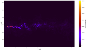 |
Figure 1: Point source release simulation in GRAL model over the area where the release test experiment was held. Figure by courtesy of Randulph |
Figure 2: Simulation in MicroHH of an elevated point source release in neutral turbulent flow over flat terrain |
During my visit to Empa I haven’t really used the GRAL model but Dominik, Randulph and I did set up a plan to perform DNS simulations with MicroHH and doing an Observation system simulation experiment (OSSE) which will mimic the release test experiment and be used in estimation of uncertainties which are affecting the measurements.Basically, the plan is to treat the simulation results as “nature” measurements since from the model we get all the information we need in every time step and in every point of our domain. The main point of study from the OSSE will be the influence of the wind on the plume dispersion and on the background concentration variations which can have a great influence on the measurements if the uncertainties are of the same order as the measured plume. Randulph will perform simulations with the same set-up in GRAL as I will do in MicroHH and later we will compare results from both models with OSSE and the measurements. At the time only ground releases were possible in MicroHH so we couldn’t do the simulations before the possibility to change the position of the source in the domain was developed.
The rest of my visit was spent looking at the data from the release test experiment done at the first MEMO2 school in February this year. We hoped to develop a useful Python code that would be able to recognize multiple measurement transects through the same plume. The measurements were done by instruments placed in moving cars and their movement was recorded by GPS so the idea was to use those to “automatize” the separation of plumes in the data file. Unfortunately, the project wasn’t finished due to time constraints, but I did get a chance to look at and work with the raw data from the Picarro instrument which, as a modeler, you don’t have a chance to do so often. So I really appreciated the experience.
I had a wonderful time in Switzerland and have enjoyed everything from meeting and working with wonderful people to exploring Zurich.
In absence of nice pictures from the Switzerland for this blog (I have never been a picture taking person) I made a small video of release of methane from an elevated point source in a turbulent flow (following the Moser example of a chanell flow). The video shows a planar view on the centerline of the plume where the longer axis is x, and the shorter is y. It can be noticed that after the plume reaches the end of the domain it reenters it on the other side and interferes with itself. This is caused by MicroHHs cyclic boundary condition and has been fixed in the latest version.